To design a register machine, we must design its data paths (registers and operations) and the controller that sequences these operations. To illustrate the design of a simple register machine, let us examine Euclid's Algorithm, which is used to compute the greatest common divisor (GCD) of two integers. As we saw in section 1.2.5, Euclid's Algorithm can be carried out by an iterative process, as specified by the following procedure: function:
| Original | JavaScript |
| (define (gcd a b) (if (= b 0) a (gcd b (remainder a b)))) | function gcd(a, b) { return b === 0 ? a : gcd(b, a % b); } |
A machine to carry out this algorithm must keep track of two numbers,
$a$ and $b$, so let us
assume that these numbers are stored in two registers with those names. The
basic operations required are testing whether the contents of register
b is zero and computing the remainder of the
contents of register a divided by the contents
of register b.
The remainder operation is a complex process, but assume for the moment that
we have a primitive device that computes remainders. On each cycle of the
GCD algorithm, the contents of register a must
be replaced by the contents of register b, and
the contents of b must be replaced by the
remainder of the old contents of a divided by
the old contents of b. It would be convenient
if these replacements could be done simultaneously, but in our model of
register machines we will assume that only one register can be assigned a
new value at each step. To accomplish the replacements, our machine will use
a third temporary
register, which we call
t. (First the remainder will be placed in
t, then the contents of
b will be placed in
a, and finally the remainder stored in
t will be placed in
b.)
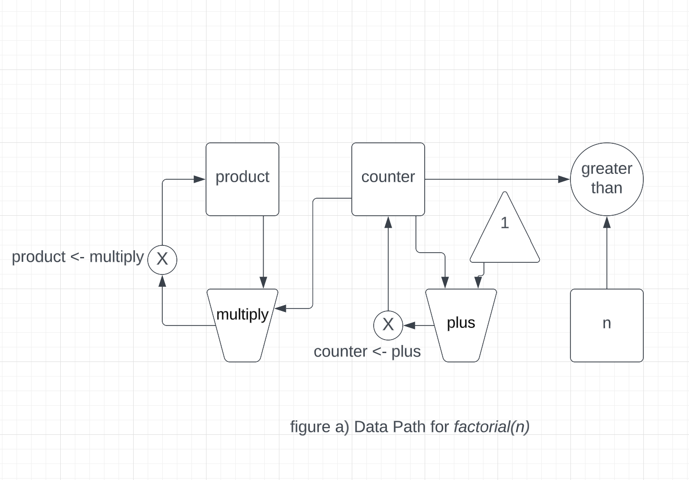
We can illustrate the registers and operations required for this
machine by using the
data-path diagram shown in
figure 5.1. In this
diagram, the registers (a,
b, and t) are
represented by rectangles. Each way to assign a value to a register is
indicated by an arrow with an Xa button—drawn as $\otimes$— behind the
head, pointing from the source of data to the register.
We can think of the X as a button that, when pushed,When pushed, the button allows
the value at the source to flow
into the designated register.
The label next to each button is the name we will use to refer to the
button. The names are arbitrary, and can be chosen to have mnemonic value
(for example, a<-b denotes pushing the
button that assigns the contents of register b
to register a). The source of data for a
register can be another register (as in the
a<-b assignment), an operation result (as in
the t<-r assignment), or a constant
(a built-in value that cannot be changed, represented in a data-path
diagram by a triangle containing the constant).
An operation that computes a value from constants and the contents
of registers is represented in a data-path diagram by a trapezoid
containing a name for the operation. For example, the box marked
rem in
figure 5.1 represents an operation that
computes the remainder of the contents of the registers
a and b to which
it is attached. Arrows (without buttons) point from the input registers and
constants to the box, and arrows connect the operation's output value
to registers. A test is represented by a circle containing a name for the
test. For example, our GCD machine has an operation that tests whether the
contents of register b is zero. A
test also has arrows from its input
registers and constants, but it has no output
arrows; its value is used by the controller rather than by the data
paths. Overall, the data-path diagram shows the registers and
operations that are required for the machine and how they must be
connected. If we view the arrows as wires and the
X$\otimes$ buttons as switches, the data-path diagram
is very like the wiring diagram for a machine that could be constructed
from electrical components.

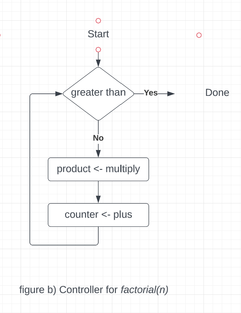
In order for the data paths to actually compute GCDs, the buttons must
be pushed in the correct sequence. We will describe this sequence in
terms of a
controller diagram, as illustrated in
figure 5.2. The elements of the
controller diagram indicate how the data-path components should be operated.
The rectangular boxes in the controller diagram identify data-path buttons
to be pushed, and the arrows describe the sequencing from one step to the
next. The diamond in the diagram represents a decision. One of the two
sequencing arrows will be followed, depending on the value of the data-path
test identified in the diamond. We can interpret the controller in terms
of a physical analogy: Think of the diagram as a maze in which a marble is
rolling. When the marble rolls into a box, it pushes the data-path button
that is named by the box. When the marble rolls into a decision node (such
as the test for
b$\, =0$), it leaves
the node on the path determined by the result of the indicated test.
Taken together, the data paths and the controller completely describe
a machine for computing GCDs. We start the controller (the rolling
marble) at the place marked start, after
placing numbers in registers a and
b. When the controller reaches
done, we will find the value of the GCD in
register a.

| Original | JavaScript |
| (define (factorial n) (define (iter product counter) (if (> counter n) product (iter (* counter product) (+ counter 1)))) (iter 1 1)) | function factorial(n) { function iter(product, counter) { return counter > n ? product : iter(counter * product, counter + 1); } return iter(1, 1); } |